Bayesian filtering
Bayesian filtering is a general framework for estimating the hidden state of a dynamical system from partial observations using a predictive model of the system dynamics.
The state, usually augmented by the system’s parameters, changes in time according to a stochastic process, and the observations are assumed to contain random noise. The goal of Bayesian filtering is to update the probability distribution of the system’s state whenever new observations become available, using the recursive Bayes’ theorem.
This section describes the theoretical background of Bayesian filtering. Interested in how GrainLearning provides parameter values to your software? Then browse directly to the sampling module.
Bayes’ theorem
Humans are Bayesian machines, constantly using Bayesian reasoning to make decisions and predictions about the world around them. Bayes’ theorem is the mathematical foundation for this process, allowing us to update our beliefs in the face of new evidence,
Note
\(p(A|B)\) is the posterior probability of hypothesis \(A\) given evidence \(B\) has been observed
\(p(B|A)\) is the likelihood of observing evidence \(B\) given hypothesis \(A\)
\(p(A)\) is the prior probability of hypothesis \(A\)
\(p(B)\) is a normalizing constant that ensures the posterior distribution sums to one
At its core, Bayes’ theorem is a simple concept: the probability of a hypothesis given some observed evidence is proportional to the product of the prior probability of the hypothesis and the likelihood of the evidence given the hypothesis. Check this video for a more intuitive explanation.
The inference module
The inference module contains classes that infer the probability
distribution of model parameters from observation data.
This process is also known as inverse analysis or data assimilation.
The output of the inference module is the probability distribution over the model state \(\vec{x}_t\),
usually augmented by the parameters \(\vec{\Theta}\), conditioned on the observation data \(\vec{y}_t\) at time \(t\).
Sequential Monte Carlo
The method currently available for statistical inference is Sequential Monte Carlo.
It recursively updates the probability distribution of the augmented model state
\(\hat{\vec{x}}_T=(\vec{x}_T, \vec{\Theta})\) from the sequences of observation data
\(\vec{y}_{0:T}\) from time \(t = 0\) to \(T\).
The posterior distribution of the augmented model state is approximated by a set of samples,
where each sample instantiates a realization of the model state.
.. Samples are drawn from a proposal density, which can be either
.. informative
.. or non-informative.
Via Bayes’ rule, the posterior distribution of the augmented model state reads
Where \(p(\hat{\vec{x}}_0)\) is the initial distribution of the model state. We can rewrite this equation in the recursive form, so that the posterior distribution gets updated at every time step \(t\).
Where \(p(\vec{y}_t|\hat{\vec{x}}_t)\) and \(p(\hat{\vec{x}}_t|\hat{\vec{x}}_{t-1})\) are the likelihood distribution and the transition distribution, respectively. The likelihood distribution is the probability distribution of observing \(\vec{y}_t\) given the model state \(\hat{\vec{x}}_t\). The transition distribution is the probability distribution of the model’s current state \(\hat{\vec{x}}_t\) given its previous state \(\hat{\vec{x}}_{t-1}\).
Note
We apply no perturbation in the parameters \(\vec{\Theta}\) nor in the model states \(\vec{x}_{1:T}\) because the model history must be kept intact for path-dependent materials. This results in a deterministic transition distribution predetermined from the initial state \(p(\hat{\vec{x}}_0)\).
Importance sampling
The prior, likelihood, and posterior distributions can be evaluated via importance sampling. The idea is to have samples that are more important than others when approximating a target distribution. The measure of this importance is the so-called importance weight (see the figure below).
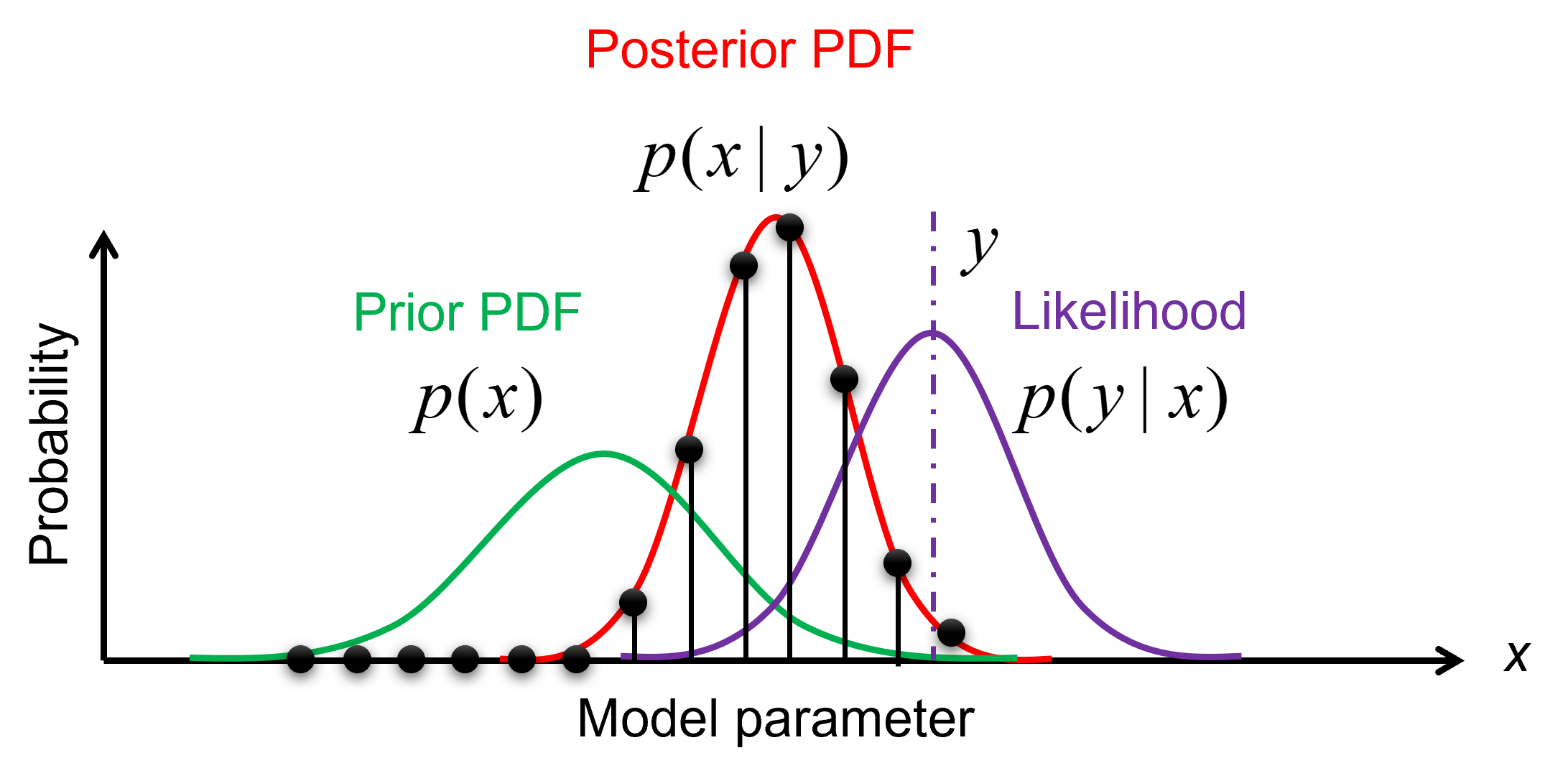
Illustration of importance sampling.
Therefore, we draw samples, \(\vec{\Theta}^{(i)} \ (i=1,...,N_p)\),
from a proposal density, leading to an ensemble of the model state \(\vec{x}_t^{(i)}\).
The importance weights \(w_t^{(i)}\) are updated recursively, via
The likelihood \(p(\vec{y}_t|\hat{\vec{x}}_t^{(i)})\)
can be assumed to be a multivariate Gaussian (see the equation below), which is computed by the function get_likelihoods
of the SMC class.
where \(\mathbf{H}\) is the observation model that reduces to a diagonal matrix for uncorrelated observables,
and \(\mathbf{\Sigma}_t^D\) is the covariance matrix cov_matrices
calculated from \(\vec{y}_t\) and the user-defined normalized variance sigma_max, in the function get_covariance_matrices.
By making use of importance sampling, the posterior distribution
\(p(\vec{y}_t|\hat{\vec{x}}_t^{(i)})\) gets updated over time in data_assimilation_loop
— this is known as Bayesian updating.
Figure below illustrates the evolution of a posterior distribution over time.
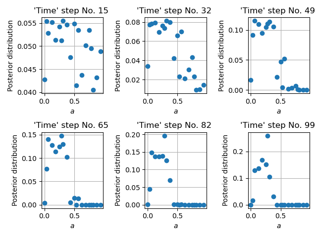
Time evolution of the importance weights over model parameter \(a\).
Ensemble predictions
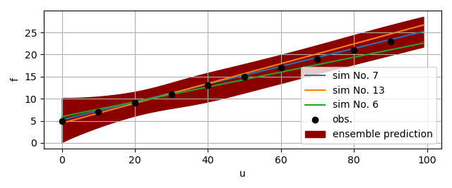
Since the importance weight on each sample \(\vec{\Theta}^{(i)}\) is discrete and the sample \(\vec{\Theta}^{(i)}\) and model state \(\vec{x}_t^{(i)}\) have one-to-one correspondence, the ensemble mean and variance of \(f_t\), an arbitrary function of the model’s augmented state \(\hat{\vec{x}}_t\), can be computed as
The figure below gives an example of the ensemble prediction in darkred, the top three fits in blue, orange, and green, and the observation data in black.
The sampling module
The sampling module allows drawing samples from
a non-informative uniform distribution
an informative proposal density designed and optimized to make the inference efficient
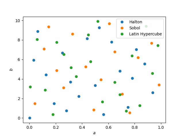
Sampling from low-discrepancy sequences
Since we typically don’t know the prior distribution of model parameters, we start with a non-informative, uniform sampling using quasi-random or near-random numbers. We make use of the Quasi-Monte Carlo generators of scipy.
You can choose one of the sampling methods when initializing a IterativeBayesianFilter object.
“sobol”: a Sobol sequence
“halton”: a Halton sequence
“LH”: a Latin Hypercube
ibf_cls = IterativeBayesianFilter.from_dict(
    {
        "inference":{
            "ess_target": 0.3,
        },
        "sampling":{
            "max_num_components": 1
        }
        "initial_sampling": "halton"
    }
)
The figure below shows parameter samples generated using a Halton sequence, a Sobol sequence and a Latin Hypercube in 2D.
Sampling from a proposal density function
An initial uniform sampling is unbiased, but it can be very inefficient since the correlation structure is not sampled.
If we have some vague idea of the posterior distribution, we can come up with a proposal density.
For that, we can use the GaussianMixtureModel class which is a wrapper of BayesianGaussianMixture of scikit-learn.
Note
Note that BayesianGaussianMixture is based on a variational Bayesian estimation of a Gaussian mixture, meaning the parameters of a Gaussian mixture distribution are inferred. For example, the number of components is optimized rather than an input of the Gaussian mixture.
The non-parametric Gaussian mixture can be trained using the previously generated samples
and their importance weights estimated by the inference method.
New samples are then drawn from this mixture model that acts as a proposal density in regenerate_params.
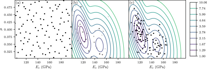
Resampling of parameter space via a Gaussian mixture model.
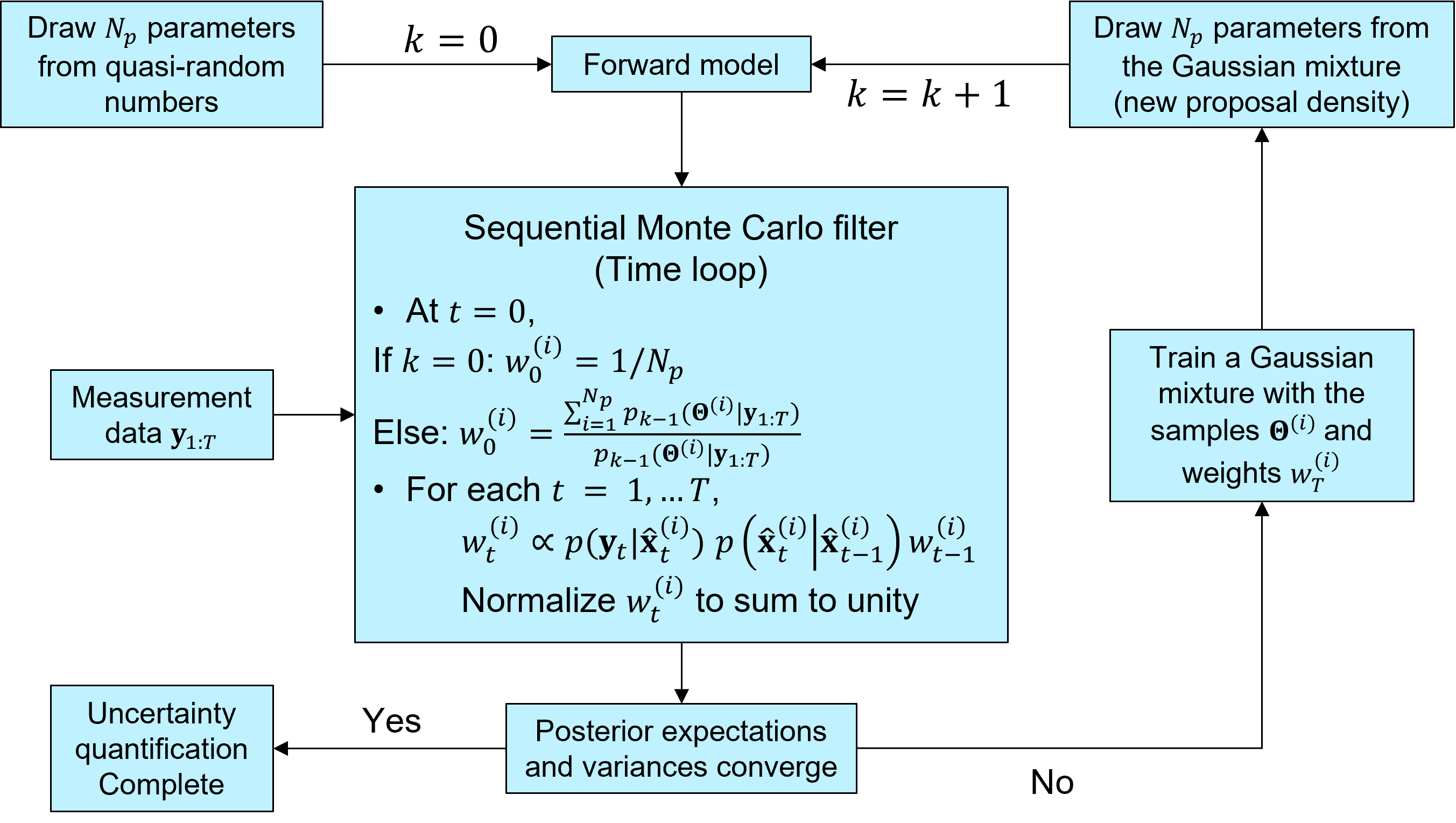
Iterative Bayesian filter
The idea of iterative Bayesian filtering algorithm is to solve the inverse problem all over again, with new samples drawn from a more sensible proposal density, leading to a multi-level resampling strategy to avoid weight degeneracy and improve efficiency. The essential steps include
Generating the initial samples using
a low-discrepancy sequence,Running the instances of the predictive (forward) model via a user-defined callback function,
Estimating the time evolution of
the posterior distribution,Generating new samples from
the proposal density, trained with the previous ensemble (i.e., samples and associated weights),Check whether the posterior expecation of the model parameters has converged to a certain value, and stop the iteration if so.
If not, repeating step 1–5 (combined into the function
IterativeBayesianFilter.solve)
Warning
When running SMC filtering via IterativeBayesianFilter.run_inference,
it is crucial to ensure that the effective sample size is large enough,
so that the ensemble does not degenerate into few samples with very large weights.
The figure below illustrates the workflow of iterative Bayesian filtering.