RNN Module

We implemented a Recurrent Neural Network (RNN) model in the tensorflow framework. For more information about the model go to section The RNN model.

There are four main usages of the RNN module:

1. Train a RNN with your own data.

2. Make a prediction with a pre-trained model.

3. Use a trained RNN model in grainLearning calibration process.

Train a RNN with your own data

Get your data to our format

The RNN model of this module considers a specific data format and organization. Our example of data consists of several DEM simulations of Triaxial Compressions of granular material specimens having different contact parameters. Such simulations were performed using YADE that outputs the simulation state to a .npy file every given amount of time steps. The files are stored under the folder structure pressure/experiment_type.

• Prepare your parsing script. We recommend to copy this script locally.

• Use CONTACT_KEYS, INPUT_KEYS and OUTPUT_KEYS consistent with your dataset. You can modify, add or remove elements of such dictionaries. These will also be stored as dataset attributes.

• Go to function main() and adapt the parameters to your own case.

  • sequence_length: The model will only work with sequences of the same size. Shorter sequences in the dataset will not be considered and longer will be trimmed to sequence_length.

  • stored_in_subfolders = True: YADE files (.npy) stored in subfolders pressure/experiment_type. The elements in lists pressure and experiment_types should be the same of your folders.

  • stored_in_subfolders = False: All your data (YADE .npy files) is stored in a single folder. You can define the pressures manually as list, such as for the first option. Or you can gather all confining pressures in your dataset via get_pressures().

  The .hdf5 file is generated with groups of pressure and experiment_type combinations. For more information about the parameters take a look at the dataset attributes API documentation [TODO].

• Use the script rnn/data_parsing/triaxial_YADE.py to read the .npy files in data_dir and create target_file with hdf5 format.

• If your data comes from another software or is stored differently please write your own parser such that the format of target_file has the structure of the one given as example.

Structure of the generated hdf5 file

• Database groups

  The data is organized in HDF5 groups with the following hierarchy:

|-- triaxial_compression.hdf5  # root
    |-- pressure               # confinement pressure
        |-- experiment_type    # drained/undrained
            |-- contact_params # dataset: no subgroup
            |-- inputs         # dataset: no subgroup
            |-- outputs        # dataset: no subgroup

You can access groups and datasets:

>>> import h5py
>>> your_hdf5_file_loaded_in_python = h5py.File('triaxial_compression.hdf5', 'r')
>>> contact_params = your_hdf5_file_loaded_in_python['0.2e6/drained/contact_params'] # HDF5 dataset
>>> contact_params = your_hdf5_file_loaded_in_python['0.2e6']['drained']['contact_params'] # HDF5 dataset, equivalent to the line above
>>> list(contact_params) # convert it to a python list
>>> contact_params[:]    # equivalent code to the line above

• Dataset attributes

  Attributes are self-explanatory strings of the meaning of each field in a dataset.

>>> import h5py
>>> your_hdf5_file_loaded_in_python = h5py.File('triaxial_compression.hdf5', 'r')
>>> attributes = your_hdf5_file_loaded_in_python.attrs
>>> attributes.keys()
>>> <KeysViewHDF5 ['contact_params', 'inputs', 'outputs', 'unused_keys_constant', 'unused_keys_sequence']>
>>> attributes['contact_params']
>>> array(['E', 'v', 'kr', 'eta', 'mu'], dtype=object)

Understand how data is prepared

Prior to training we do some manipulation of the numpy arrays stored in the hdf5 database to get them to tensorflow datasets. The main transformations involve: merging arrays from different hdf5 groups, standardizing the data, splitting de dataset in train, validation and test datasets, including or excluding information from the hdf5 group name to the parameters passed to the neural network.

We have an abstract class Preprocessor and a child class PreprocessorTriaxialCompression with the implementation of the abstract methods tailored to the case of Triaxial Compression DEM simulations. At the moment, this one considers the Sliding windows technique for handling the data during training and prediction.

Option 1: Train using wandb

Weights a Biases is an external platform that can be used for tracking experiments and hyperparameter tuning. It allows the user to gather training metrics, model configuration and system performance for different runs (i.e. training of your RNN).

To use it you have to create a free account. If you have installed grainLearning with rnn dependencies, wandb should be already in your system, otherwise, you can install it: pip install wandb.

For both single runs and sweeps, wandb will create a folder named wandb containing metadata and files generated during the run(s). In this same folder, per each run, you will find 3 files: config.yaml, train_stats_npy and model-best.h5. These files contain all the information required to load your model in the future.

Warning

You can run your training on offline model with wandb, but in that case config.yaml will not be generated until you sync your files. If you don’t want to sync the files or create an account on wandb, consider using Option 2: Train using plain tensorflow.

Experiment tracking: Single run

Create my_train.py where you would like to run the training. Be aware to configure the data directory accordingly (See API docs for more information about the config keys). Avoid creating this file inside the grainlearning package nor rnn module.

my_train.py

import grainlearning.rnn.train as train_rnn
from grainlearning.rnn import preprocessor

# 1. Create my dictionary of configuration
my_config = {
     'raw_data': 'path_to_dataset.hdf5',
     'pressure': 'All',
     'experiment_type': 'drained',
     'add_pressure': True,
     'add_e0': True,
     'train_frac': 0.7,
     'val_frac': 0.15,
     'window_size': 20,
     'window_step': 1,
     'patience': 25,
     'epochs': 10,
     'learning_rate': 1e-4,
     'lstm_units': 250,
     'dense_units': 250,
     'batch_size': 256,
     'standardize_outputs': True,
     'save_weights_only': True
 }

# 2. Create an object Preprocessor to pre-process my data
preprocessor_TC = preprocessor.PreprocessorTriaxialCompression(**my_config)

# 3. Run the training Tensorflow and reporting to wandb
train_rnn.train(preprocessor_TC, config=my_config)

Open a terminal where you have your file, activate the environment where grainLearning and rnn dependencies has been installed and run: python my_train.py

If is the first time running wandb it will ask you to login (copy paste your API key that you’ll find in your wandb profile).

In this example we used a default configuration, but you can define your own config dictionary. For more info go to our Python API-RNN-train.

Hyperparameter optimization: Sweep

Wandb Sweeps allows the user to train the model with different hyperparameters combinations gathering metrics in the wandb interface to facilitate the analysis and choice of the best model.

You can run your sweep:

• From a python file.

• From the command line.

From a python file

Create my_sweep.py where you would like to run the training. Configure the sweep parameters (See API docs for more information about the config keys). Avoid creating this file inside the grainlearning package nor rnn module. See this for more information about sweep configuration, and this wandb guide.

my_sweep.py

import wandb
import grainlearning.rnn.train as train_rnn
from grainlearning.rnn import preprocessor

def my_training_function():
  """ A function that wraps the training process"""
  preprocessor_TC = preprocessor.PreprocessorTriaxialCompression(**wandb.config)
  train_rnn.train(preprocessor_TC)

if __name__ == '__main__':
   wandb.login()
   sweep_configuration = {
   'method': 'bayes',
   'name': 'sweep',
   'metric': {'goal': 'maximize', 'name': 'val_acc'},
   'parameters':
      {
      'raw_data': 'my_path_to_dataset.hdf5',
      'pressure': 'All',
      'experiment_type': 'All',
      'add_e0': False,
      'add_pressure': True,
      'add_experiment_type': True,
      'train_frac': 0.7,
      'val_frac': 0.15,
      'window_size': 10,
      'window_step': 1,
      'pad_length': 0,
      'lstm_units': 200,
      'dense_units': 200,
      'patience': 5,
      'epochs': 100,
      'learning_rate': 1e-3,
      'batch_size': 256,
      'standardize_outputs': True,
      'save_weights_only': False
      }
   }

   # create a new sweep, here you can also configure your project and entity.
   sweep_id = wandb.sweep(sweep=sweep_configuration)

   # run an agent
   wandb.agent(sweep_id, function=my_training_function, count=4)

Open a terminal where you have your file, activate the environment where grainLearning and rnn dependencies has been installed and run: python my_sweep.py.

If you want to run another agent or re-start the sweep you can replace the creation of a new step sweep for assigning the id of your sweep to the variable sweep_id.

From the command line

1. Configure your sweep:

   In folder sweep example_sweep.yaml contains the sweep configuration values and/or range of values per each hyperparameter. You can choose as many values and in which ranges wandb will search for the optimal combination.

   Don’t forget to put your own project and entity to get the results in your wandb dashboard. For more information about how to configure the .yaml file see this.

   Note

   The combination of values of the parameter that wandb is going to draw for each run will override those of the default dictionary in train.py.

2. Create a copy of example_sweep.yaml outside grainlearning package and rnn module, in the folder where you want to run your sweep.

3. wandb` folder containing the runs information an model data will be automatically created in this folder. Change raw_data value accordingly.

4. Create python file my_sweep_CL.py and in example_sweep.yaml set program: my_sweep_CL.py.

my_sweep_CL.py

import grainlearning.rnn.train as train_rnn
from grainlearning.rnn import preprocessor

wandb.init()
preprocessor_TC = preprocessor.PreprocessorTriaxialCompression(**wandb.config)
train_rnn.train(preprocessor_TC)

4. Open a terminal and activate the environment where grainLearning and rnn dependencies are installed.

5. If you are running the training in a supercomputer continue with the instructions in Running a Sweep on HPC.

6. Create a sweep: wandb sweep example_sweep.yaml.

   This will print out in the console the sweep ID as well as the instructions to start an agent.

7. Run an agent: wandb agent <entity>/<project>/<sweep_id>.

   Running this command will start a training run with hyperparameters chosen according to example_sweep.yaml, will keep starting new runs, and will update your wandb dashboard. Models are saved both locally and also uploaded to wandb.

Running a Sweep on HPC

Warning

This instructions assume that your HPC platform uses job scheduler slurm. run_sweep.sh configures the job and loads modules from Snellius, these can be different in other supercomputers.

1. Install grainLearning and rnn dependencies.

2. Create the folder containing your data, run_sweep.sh, file my_sweep_CL.py and example_sweep.yaml, make sure to modify the last one accordingly.

3. Check that run_sweep.sh load the correct modules. In this file the outputs of the job will be directed to job_outputs. It can be that in your HPC such folder is not automatically created and thus, you have to do it before running your script.

4. Run your job: sbatch run_sweep.sh This command will create the sweep, gather the sweep_id from the output that is printed on the terminal and then start an agent.

Option 2: Train using plain tensorflow

Create my_train.py where you would like to run the training. Be aware to configure the data directory accordingly. Avoid creating this file inside the grainlearning package nor rnn module.

my_train.py

import grainlearning.rnn.train as train_rnn
from grainlearning.rnn import preprocessor

# 1. Create my dictionary of configuration
my_config = {
     'raw_data': 'path_to_dataset.hdf5',
     'pressure': 'All',
     'experiment_type': 'drained',
     'add_pressure': True,
     'add_e0': True,
     'train_frac': 0.7,
     'val_frac': 0.15,
     'window_size': 20,
     'window_step': 1,
     'patience': 25,
     'epochs': 10,
     'learning_rate': 1e-4,
     'lstm_units': 250,
     'dense_units': 250,
     'batch_size': 256,
     'standardize_outputs': True,
     'save_weights_only': True
 }

# 2. Create an object Preprocessor to pre-process my data
preprocessor_TC = preprocessor.PreprocessorTriaxialCompression(**my_config)

# 3. Run the training using bare tensorflow
train_rnn.train_without_wandb(preprocessor_TC, config=my_config)

Open a terminal where you have your file, activate the environment where grainLearning and rnn dependencies has been installed and run: python my_train.py

The folder outputs is created containing config.npy, train_stats.npy and either saved_model.pb or weights.h5 depending if you choose to save the entire model or only its weights. The contents of this directory will be necessary to load the trained model in the future.

Warning

Every time you run a new experiment the files in outputs will be override. If you want to save them, copy them to another location once the run is finished.

Make a prediction with a pre-trained model

You can load a pre-trained model from:

• Saved model.

• A wandb sweep.

Saved model

You can find some pre-trained models in in rnn/train_models and you can also load a model that you have trained. The function get_pretrained_model() will take care of checking if your model was trained via wandb or outside of it, as well as if only the weights were saved or the entire model.

In this example, we are going to load the same dataset that we used for training, but we are going to predict from the test sub-dataset. Here you’re free to pass any data having the same format (tf.data.Dataset) and respecting the input dimensions of the model:

predict_from_pre-trained.py

from pathlib import Path

import grainlearning.rnn.predict as predict_rnn
from grainlearning.rnn import preprocessor

# 1. Define the location of the model to use
path_to_trained_model = Path('C:/trained_models/My_model_1')

# 2. Get the model information
model, train_stats, config = predict_rnn.get_pretrained_model(path_to_trained_model)

# 3. Load input data to predict from
config['raw_data'] = '../train/data/my_database.hdf5'
preprocessor_TC = preprocessor.PreprocessorTriaxialCompression(**config)
data, _ = preprocessor_TC.prepare_datasets()

#4. Make a prediction
predictions = predict_rnn.predict_macroscopics(model, data['test'], train_stats, config,batch_size=256, single_batch=True)

If the model was trained with standardize_outputs = True, predictions are going to be unstandardized (i.e. no values between [0, 1] but with the original scale). In our example, predictions is a tensorflow tensor of size (batch_size, length_sequences - window_size, num_labels).

A wandb sweep

You need to have access to the sweep and know its ID. Often this looks like <entity>/<project>/<sweep_id>.

predict_from_sweep.py

from pathlib import Path

import grainlearning.rnn.predict as predict_rnn
from grainlearning.rnn import preprocessor

# 1. Define which sweep to look into
entity_project_sweep_id = 'grainlearning-escience/grainLearning-grainlearning_rnn/6zrc0vjb'

# 2. Chose the best model from a sweep, and get the model information
model, data, train_stats, config = predict_rnn.get_best_run_from_sweep(entity_project_sweep_id)

# 3. Load input data to predict from
config['raw_data'] = '../train/data/sequences.hdf5'
preprocessor_TC = preprocessor.PreprocessorTriaxialCompression(**config)
data, _ = preprocessor_TC.prepare_datasets()

#4. Make a prediction
predictions = predict_rnn.predict_macroscopics(model, data['test'], train_stats, config,batch_size=256, single_batch=True)

This can fail if you have deleted some runs or if your wandb folder is not present in this folder. We advise to copy config.yaml, train_stats.py and model_best.h5 from wandb/runXXX/files to another location and follow Saved model instructions. These files can also be downloaded from the wandb dashboard.

Use a trained RNN model in grainLearning calibration process

A trained RNN can be used as a surrogate model and play the role of a DynamicSystem in the calibration workflow. In such case, instead of having to generate your data in advance or performing a complete DEM simulation per iteration and group of parameters, the simulation data is provided by the RNN.

In which cases can we use RNN for the calibration process?

Warning

We recommend you to be careful when using Neural Networks as surrogate models, always check and test your workflows, be mindful of the I) parameters that you pass to your Neural Network, and II) model capabilities.

• You have several simulation and/or experimental data in which you clearly identify: - Control parameters that may vary during the experiment (i.e. system.ctrl_data). - Tunable parameters that remain constant during the experiment and can be inferred through the calibration process (i.e. system.param_data). - Observation parameters that evolve during the experiment and are not controlled (i.e. system.sim_data), for example the material response.

• You need several data because the performance (both accuracy and generalization) of the RNN depends on how much data was it trained on. No-one would like to rely their calibration process on an RNN that performs well only for a very-specific set of parameters.

• Your time sequences have always the same length. Both for GrainLearning and RNN models this dimension of the data must be fixed. Considering handling your data such that you trim the vectors to the same length.

• Consistency is key: understand the dimensions of your data, if it need to be normalized, and if it is consistent with what the pre-trained model is expecting.

How does it work?

A simple example can be found in tutorials. Such tutorial has three main parts:

1. Prepare the pre-trained model: Load a model using grainlearning.rnn.predict.get_pretrained_model().

2. Create a callback function to link to `BayesianCalibration`: Function in which the predictions are going to be drawn.

3. GrainLearning calibration loop.

In this case, synthetic data was considered: we took one example from our triaxial compression DEM simulations. This is useful to show the functionality since we know in advance the desired output. However, in a real-world case, one may have an RNN trained on DEM simulations and the observation is an experiment of an equivalent system. In that case, most_prob_params inferred by grainlearning correspond to the contact_params of the DEM simulation being equivalent to your real-world material.

Tips

• The inputs to the RNN are:

  • load_sequence: system.ctrl_data and

  • contact_params: system.param_data.

  And system.set_sim_data() should be called with the outputs (i.e prediction) of the RNN.

• Set the ranges defined by param_min and param_max of the as the system to the ranges in which you understand how your trained model performs.

The RNN model

The RNN model is a Neural Network with RNN layer implemented in Tensorflow. We consider the case of a Triaxial compressions of granular materials simulated using DEM.

• Inputs: Load time sequence of size (sequence_length, num_load_features) (e.g. strains in x, y, z) and num_contact_params contact parameters.

• Outputs: Time sequences of num_labels macroscopic variables such as the stress and void ratio.

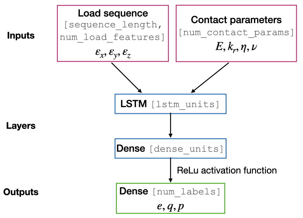
Note

• lstm_units, dense_units: Hyperparameters requiring tuning when training a model.

• sequence_length, num_load_features, num_contact_params, num_labels: sizes determined by the data.

The contact parameters are first passed through 2 trainable dense layers whose outputs are state_h and state_c. Such outputs are the initial state of the LSTM layer.

Note

num_contact_params, num_load_features and num_labels are determined during the preparation of your data and depending on the choice of Preprocessor, they may be different. CHeck the documentation of the Preprocessor that you use.

Sliding windows

The data is split along the temporal dimension in sliding windows of fixed length window_size. In essence, the input for the RNN model is a window of inputs (window_i in the figure below) and the prediction is the last element in the equivalent window in the sequence of outputs (output_i in the figure below).

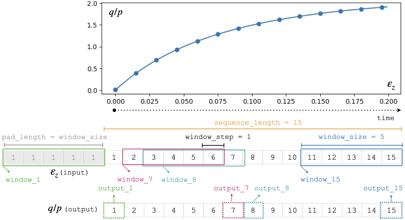
The module takes care of splitting the data into windows and stacking the predictions for each step of the sequence. With this configuration, the first window_size points are not predicted by the model. To predict those too, add pad_length equals to window_size to the config dictionary. The trick here will be to add pad_length copies of the first element of inputs to the sequence that will be afterwards windowized.

Note

• window_size is a hyperparameter requiring tuning when training a model.

• sequence_length is fixed by the user. All sequences in a dataset must have the same length.

• window_step is the distance (in position) between the start (or end) of consecutive windows. In general window_step = 1.

Loss and metrics

• Loss: tensorflow MSE for train and validation datasets.

• Metric: tensor flow MAE is logged for train and validation datasets.

• Optimizer: tensorflow Adam requiring the learning_rate. Other additional parameters for the optimizer can be defined config dictionary.

• Callbacks:

  • tensorflow EarlyStopping: Using patience defined in config dictionary and val_loss as monitoring metric.

  • tensorflow ModelCheckpoint: Using save_weights_only defined in config dictionary and saving best only.