Examples

This section contains various applications of GrainLearning for the Bayesian calibration of granular material models. In granular materials, plastic deformation at the macro scale arises from contact sliding in the tangential and rolling/twisting directions and the irrecoverable change of the microstructure. Because the parameters relevant to these microscopic phenomena are not directly measurable in a laboratory, calibration of DEM models is generally treated as an inverse problem using “inverse methods”, ranging from trials and errors to sophisticated statistical inference.

Solving an inverse problem that involves nonlinearity and/or discontinuity in the forward model (DEM or constitutive) is very challenging. Furthermore, because of the potentially large computational cost for running the simulations, the “trials” have to be selected with an optimized strategy to boost efficiency.

Bayesian calibration of DEM models

Run DEM simulations guided by GrainLearning

Process simulation data with GrainLearning

In the case of DEM modeling of granular soils, relevant parameters could be Young’s modulus, friction coefficient, Poisson’s ratio, rolling stiffness, and rolling friction, etc. of a soil particle, as well as structural parameters like a particle size distribution parameterized by its moments. Below is a piece of code that performs Bayesian calibration of four DEM parameters using triaxial compression data.

from grainlearning import BayesianCalibration
from grainlearning.dynamic_systems import IODynamicSystem

curr_iter = 1
sim_data_dir = './tests/data/oedo_sim_data'

calibration = BayesianCalibration.from_dict(
    {
        "curr_iter": curr_iter,
        "num_iter": 0,
        "system": {
            "system_type": IODynamicSystem,
            "obs_data_file": 'obsdata.dat',
            "obs_names": ['p','q','n'],
            "ctrl_name": 'e_a',
            "sim_name": 'oedo',
            "sim_data_dir": sim_data_dir,
            "param_data_file": f'{sim_data_dir}/iter{curr_iter}/smcTable{curr_iter}.txt',
            "param_names": ['E', 'mu', 'k_r', 'mu_r'],
            "param_min": [100e9, 0.3, 0, 0.1],
            "param_max": [200e9, 0.5, 1e4, 0.5],
            "inv_obs_weight": [1, 1, 0.01],
        },
        "calibration": {
            "inference": {"ess_target": 0.2},
            "sampling": {
            "max_num_components": 10,
            "prior_weight": 0.01,
            },
        },
        "save_fig": 0,
    }
)

#%%
# load the simulation data and run the inference for one iteration
calibration.load_and_run_one_iteration()

In this example, GrainLearning read the data from pre-run simulations stored in sim_data_dir, We control the model uncertainty to reach an effective sample size of 20%. A new parameter table is generated in the subdirectory of sim_data_dir. The following figure shows the resampled parameter sub-spaces that are progressively localized near the posterior modes over the iterations.

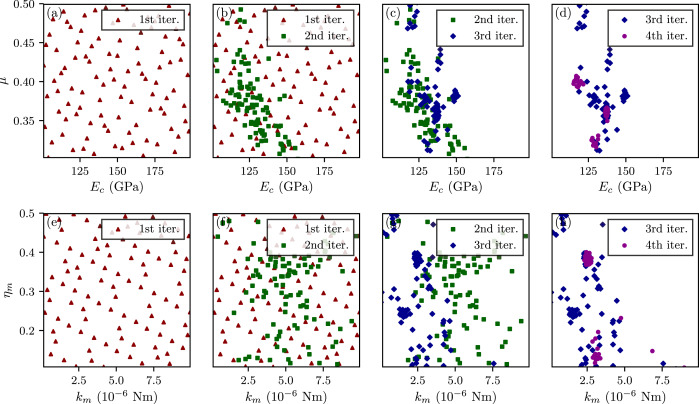
Localization of resampled parameter values over a few iterations.

Because the closer to a posterior distribution mode the higher the sample density, resampling from the repeatedly updated proposal density allows zooming into highly probable parameter subspace in very few iterations. The iterative (re)sampling scheme brings three major advantages to Bayesian filtering:

1. The posterior distribution is iteratively estimated with an increased resolution on the posterior landscape.

2. The multi-level sampling algorithm keeps allocating model evaluations in parameter subspace where the posterior probabilities are expected to be high, thus significantly improving computational efficiency.

3. Resampling that takes place between two consecutive iterations can effectively overcome the weight degeneracy problem while keeping sample trajectories intact within the time/load history.